In a recent post I presented several equations and just as many self-starting functions for nonlinear regression analyses in R. Today, I would like to build upon that post and present some further equations, relating to the so-called threshold models.
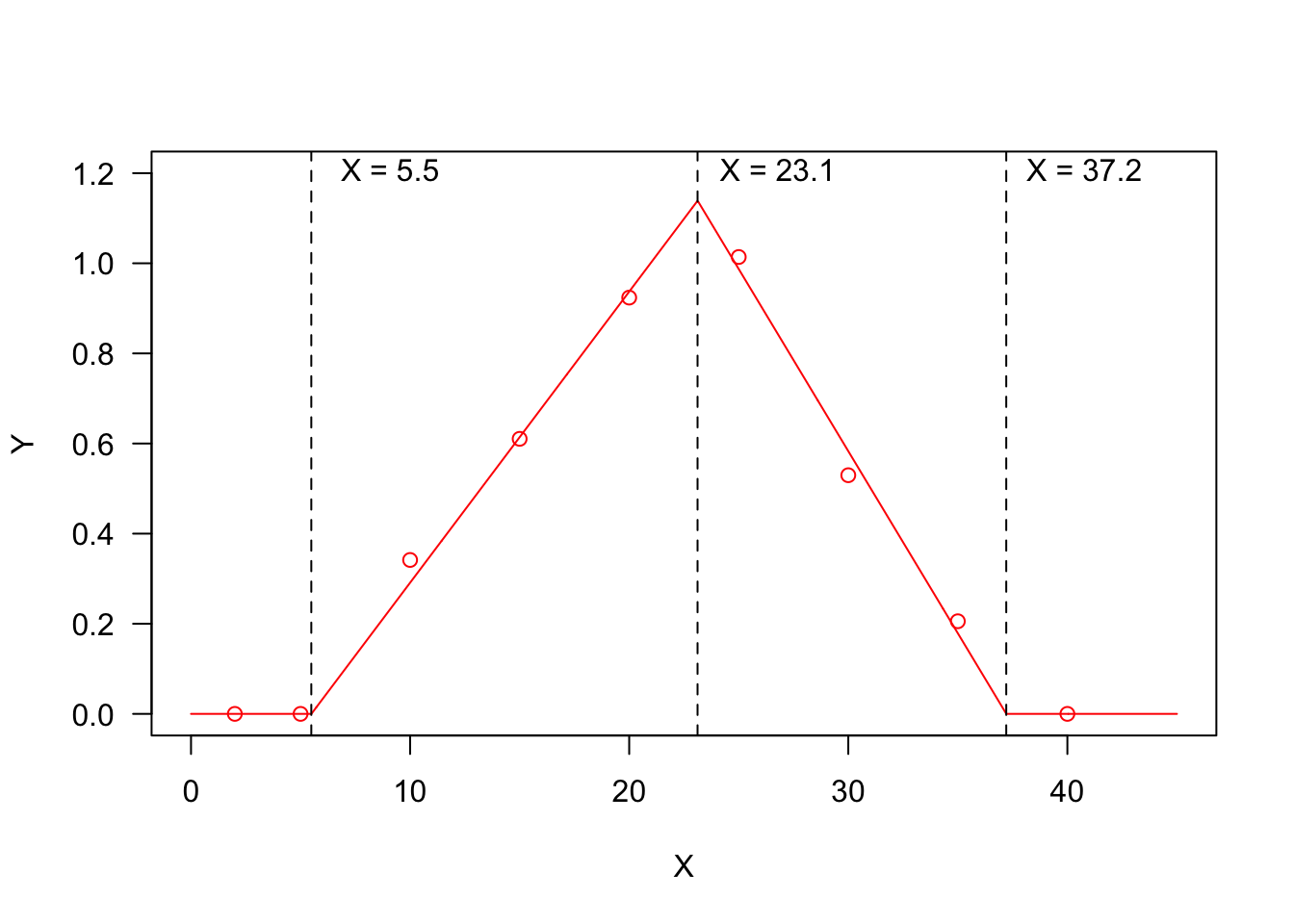
But, … what are threshold models? In some instances, we need to describe relationships where the response variable changes abruptly, following a small change in the predictor. A typical threshold model looks like that in the Figure below, where we see three threshold levels:
- X=5.5: at this threshold, the response changes abruptly from ‘flat’ to linearly increasing;
- X=23.1: at this threshold, the response changes abruptly from linearly increasing to linearly decreasing;
- X=37.2: at this threshold, the response changes abruptly from linearly decreasing to ‘flat’.
You may recognise a ‘broken-stick’ pattern, although threshold models can also be curvilinear, as we will see later.
Threshold models are very common in biology, where they can be successfully used to describe the daily (or hourly) progress towards a certain developmental stage, as influenced by the environmental conditions, mainly humidity and temperature. In this post I will show examples relating to seed germination, but the very same concepts also apply to the growth of plants and other organisms. In biology, these models are often known as thermal-time or hydro-time models.
Considering seed germination, the response variable is the Germination Rate (GR), that is the reciprocal of germination time; for example, if a seed takes 7 days to accomplish the germination process, the GR is equal to 1/7=0.143 and it represents the fraction of germination that is accomplished in one day. The GR is a good measure of velocity: the higher the value the higher the speed. If we plot the GR against, e.g., temperature, we should very likely observe a response pattern as in Figure 1; the three thresholds are, respectively, the base temperature (T_b_), the optimal temperature (T_o_) and the ceiling temperature (T_c_). If we look at the effect of soil humidity on GR, we should expect a response pattern with only one threshold, i.e. the base water potential (e.g. the first half of Figure 1, up to the maximum response level).
Although the equations I am going to introduce are commonly used in the seed science literature, I am confident that you might find them useful for a lot of other applications. For all those equations, I have built the related R functions, together with self-starting routines, which can be used for nonlinear regression analyses with the drm() function in the ‘drc’ package (Ritz et al., 2019). The availability of self-starting routines will free you from the hassle of having to provide initial guess for model parameters. All these R functions are available within the ‘drcSeedGerm’ package (Onofri, 2019).
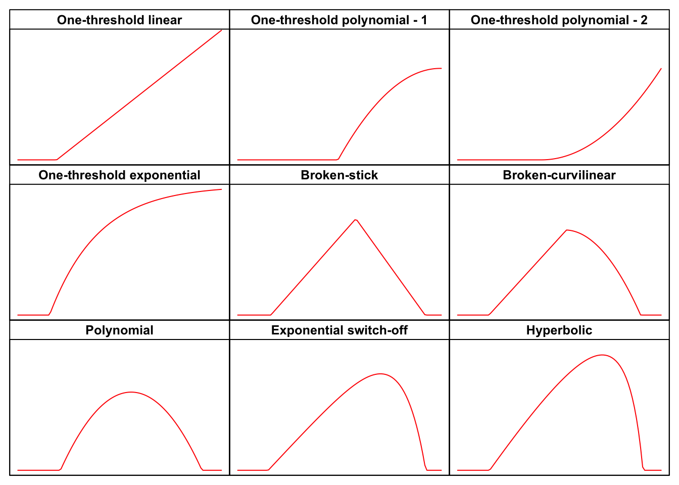
The post is rather long, but you do not need to read it all; have a look at the graph below to spot the shape you are interested in and use the link to reach the relevant part in this web page. But, first of all, do not forget to install (if necessary) and load the ‘drcSeedGerm’ package, by using the code below.
#installing package, if not yet available
# library(devtools)
# install_github("onofriandreapg/drcSeedGerm")

# loading package
library(drcSeedGerm)
List of threshold models
In this post I will show the following threshold models:
- One-threshold linear
- One-threshold polynomial - 1
- One-threshold polynomial - 2
- One-threshold exponential
- Broken-stick model
- Broken-curvilinear model
- Polynomial model
- Exponential switch-off model
- Hyperbolic model
One-threshold linear model
In some cases, we may need to model a process occurring only above a certain threshold level for the predictor variable. Models of this kind have been used to describe the effect of environmental humidity (Ψ, in MPa) on germination rate (Bradford, 2002):
GR=max
The parameter \Psi_b is the base water potential (in MPa), representing the minimum level of humidity in the substrate to trigger the germination process. The other parameter \theta_H (in MPa day or MPa hour) is the hydro-time constant.
A totally similar model has been used by Garcia-Huidobro et al (1982), to describe the effect of sub-optimal temperatures (T in °C) on the germination rate:
GR = \frac{\max \left[T, T_b\right] - T_b}{\theta_T} \quad \quad \quad \quad (2)
where T_b is the base temperature and \theta_T is the thermal time (in °C d).
Both models can be fitted in R, by using the two functions GRPsi.Lin() and GRT.GH(); they are totally equivalent, apart from parameter names. In the example below I have fitted the second equation to a seed germination dataset; this type of data is usually heteroscedastic, thus, please note the use of a robust variance-covariance estimator for model parameters (Zeileis, 2006).
Tlev <- c(2, 5, 10, 15, 20, 25)
GR <- c(0, 0, 0.21, 0.49, 0.68, 0.86)
modGH <- drm(GR ~ Tlev, fct = GRT.GH())
library(sandwich); library(lmtest)
coeftest(modGH, vcov = sandwich)
##
## t test of coefficients:
##
##                    Estimate Std. Error t value  Pr(>|t|)
## Tb:(Intercept)      4.77160    0.31993  14.915 0.0001177 ***
## ThetaT:(Intercept) 22.83118    0.62847  36.328 3.428e-06 ***
## ---
## Signif. codes:  0 '***' 0.001 '**' 0.01 '*' 0.05 '.' 0.1 ' ' 1
 r
plot(modGH, log="", xlim = c(0, 25), legendPos = c(5, 1.2),
     xlab = "Temperature (°C)")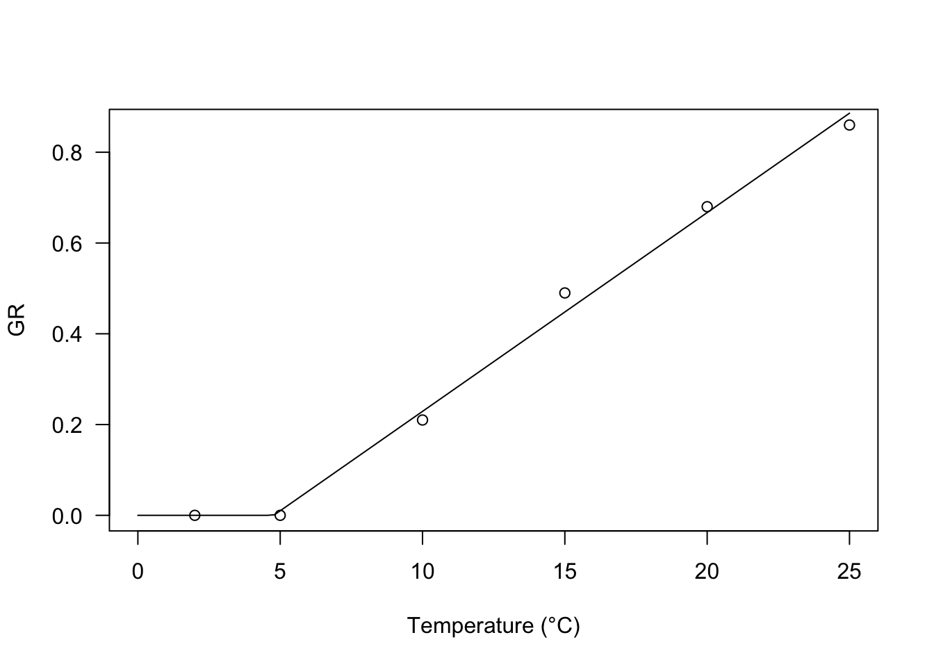
One threshold polynomial
In my experience, I have found that the relationship between GR and water potential in the substrate may, sometimes, be curvilinear. For these situations, I have successfully used the following equations:
GR = \frac{\max\left[\Psi,\Psi_b\right]^2 - \Psi^2_b}{\theta_H} \quad \quad \quad \quad (3)
and:
GR = \frac{\left(\max\left[\Psi, \Psi_b\right] - \Psi_b \right)^2}{ \theta_H } \quad \quad \quad \quad (4)
Both models can be fitted in R, by using the two functions GRPsi.Pol() and GRPsi.Pol2(), as shown in the box below.
# Observed data
Psi <- c(-2, -1.5, -1.2, -1, -0.8, -0.6, -0.4, -0.25,
         -0.12, -0.06, -0.03, 0)
GR <- c(0, 0, 0, 0, 0.0585, 0.094, 0.1231, 0.1351,
        0.1418, 0.1453, 0.1458, 0.1459)
Psi2 <- c(-0.5, -0.6, -0.7, -0.8, -0.9, -1, -1.1, -1.2,
          -1.5)
GR2 <- c(1.4018, 1.0071, 0.5614, 0.3546, 0.2293, 0, 0,
         0, 0)


modHT <- drm(GR ~ Psi, fct = GRPsiPol())
modHT2 <- drm(GR2 ~ Psi2, fct = GRPsiPol2())
par(mfrow = c(1,2))

plot(modHT, log="", legendPos = c(-1.5, 0.15),
     ylim = c(0, 0.20), xlab = "Water potential (MPa)")
plot(modHT2, log="", legendPos=c(-1.3, 1),
     xlab = "Water potential (MPa)")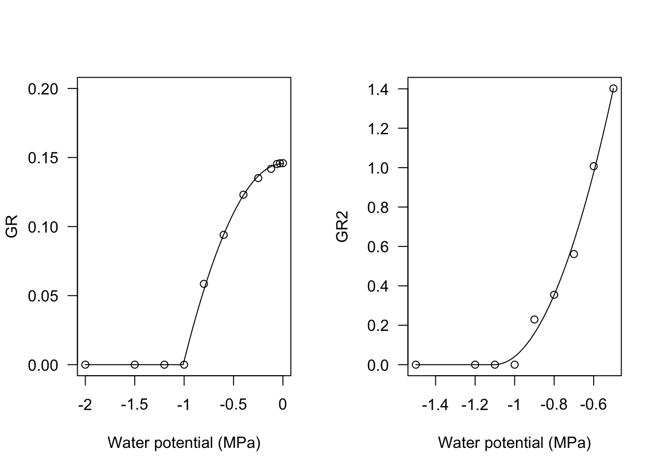
One threshold: exponential
All the previous models tend to go up to infinity when the predictor value (temperature or water potential) goes to infinity. In some instances, we may need an asymptotic model, for example, to describe the oxygen uptake kinetics during a walk test (see Baty et al., 2014, although their threshold model is more complex) or to describe the response of the maximum proportion of germinated seeds to soil humidity (Onofri et al., 2018).
In practice, we could use a shifted exponential model:
\pi = G \, \left[ 1 - exp \left( \frac{ \max\left[\Psi, \Psi_b\right] - \Psi_b }{\sigma} \right) \right] \quad \quad \quad \quad (5)
where \pi is the proportion of germinated seeds, G is the fraction of non-germinable seeds (e.g., dormant seeds) and \sigma describes how quickly the population of seeds responds to increased humidity in the substrate.
If we reverse the sign of \sigma in Eq. 5, we obtain a decreasing trend, which might be useful to describe the effect of super-optimal temperatures on the proportion of germinated seeds, going down to 0 at the ceiling temperature threshold.
Both equations can be fitted using the self-starters PmaxPsi1() and PmaxT1(). The two R functions are totally equal, apart from parameters names.
par(mfrow = c(1,2))
# Pmax vs Psi
Psi <- seq(-2.2, 0, by = 0.2)
Pmax <- c(0, 0, 0.076, 0.413, 0.514, 0.643, 0.712,
          0.832, 0.865, 0.849, 0.89, 0.90)
mod <- drm(Pmax ~ Psi, fct = PmaxPsi1())
plot(mod, log = "", xlab = "Water potential (MPa)",
     ylab = "Proportion of germinating seeds")

# Pmax vs temperture
Tval <- c(0, 2.5, 5, 7.5, 10, 12.5, 15, 17.5,
          20, 22.5, 25, 27.5, 30, 32.5, 35)
Pmax2 <- c(0.79, 0.81, 0.807, 0.776, 0.83,
           0.73, 0.744, 0.73, 0.828, 0.818,
           0.805, 0.706, 0.41, 0.002, 0)
mod2 <- drm(Pmax2 ~ Tval, fct = PmaxT1())
plot(mod2, log = "", xlab = "Temperature (°C)",
     ylab = "Proportion of germinating seeds")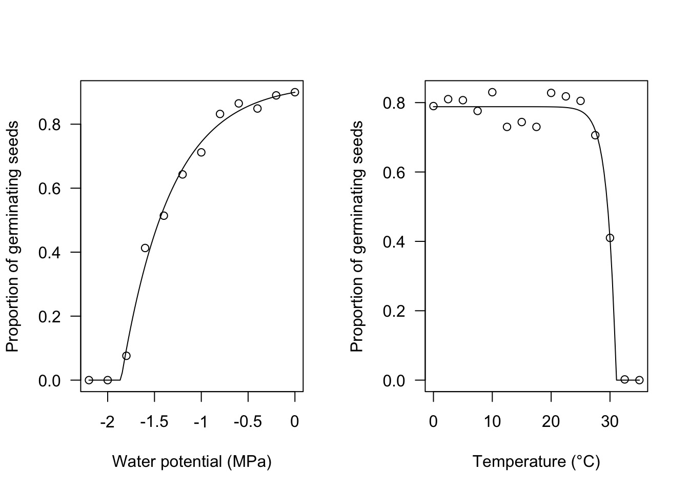
‘Broken-stick’ model
A broken-stick trend, as the one depicted in the Figure 1 was used by Alvarado and Bradford (2002) to model the effect of temperature on the germination rate. The equation is:
GR = \frac{\min \left[T,T_o \right] - T_b}{\theta_{T}} \, \left\{ 1 - \frac {\min \left[\max \left[ T,T_o \right], T_c \right] - T_o}{T_c - T_o} \right\} \quad \quad (6)
Base, optimal and ceiling temperatures (respectively T_b, T_o and T_c) are included as parameters, together with the hydro-thermal time parameter (\theta_T). Equation 6 can be easily fitted with the GRT.BS() function in the ‘drcSeedGerm’ package.
Tval <- c(2, 5, 10, 15, 20, 25, 30, 35, 40)
GR <- c(0, 0, 0.209, 0.435, 0.759, 0.821, 0.417, 0.145, 0)

modBS <- drm(GR ~ Tval, fct = GRT.BS())
plot(modBS, log="", xlim = c(0, 40), ylim=c(0,1.2),
     legendPos = c(5, 1.0), xlab = "Temperature (°C)")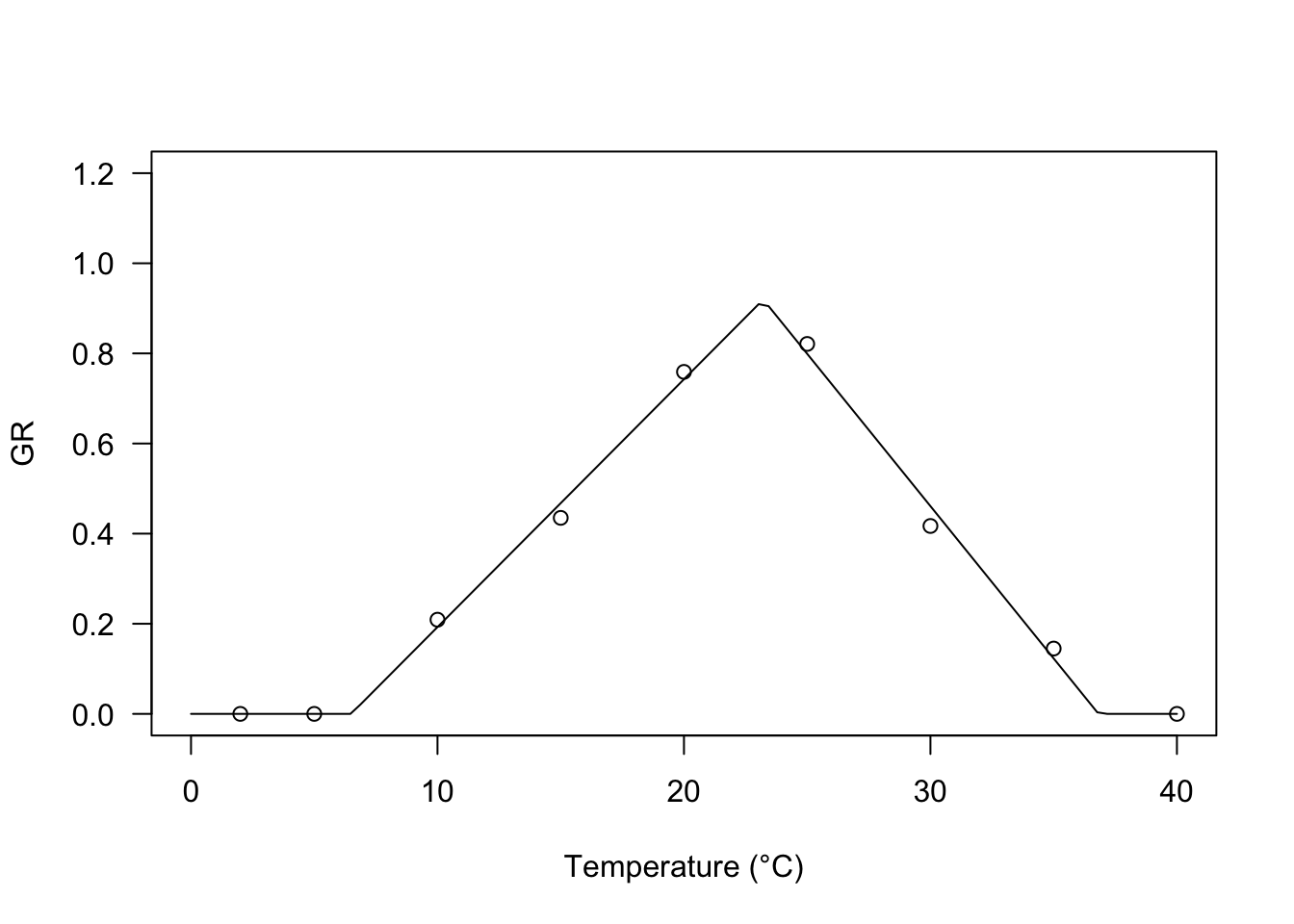
coeftest(modBS, vcov = sandwich)
##
## t test of coefficients:
##
##                     Estimate Std. Error t value  Pr(>|t|)
## k:(Intercept)       0.073515   0.002892  25.420 1.759e-06 ***
## Tb:(Intercept)      6.496708   0.431500  15.056 2.341e-05 ***
## To:(Intercept)     23.216552   0.294743  78.769 6.249e-09 ***
## ThetaT:(Intercept) 18.182167   0.763361  23.819 2.430e-06 ***
## ---
## Signif. codes:  0 '***' 0.001 '**' 0.01 '*' 0.05 '.' 0.1 ' ' 1
Broken-curvilinear model
Broken-stick trends may not be reasonable for biological processes, which might be better described by curvilinear equations. Rowse and Finch-Savage (2003) proposed another equation with two components: the first one depicts a linear increase of the GR value with temperature, which is off-set by the second component, starting from T = T_d, which is close to (but not coincident with) T_o. The equation is:
GR = \frac{ \max \left[ T, T_b \right] - T_b}{\theta_{T}} \left\{ 1 - \frac{\min \left[ \max \left[T,T_d\right], T_o \right] - T_d}{T_c - T_d} \right\} \quad \quad (7)
The optimal temperature can be derived as:
T_o = \frac{1 + kT_b + kT_d}{2k}
where:
k = \frac{1}{T_c - T_d}
For this equation, you will find the GRT.RFb() self-starter in the ‘drcSeedGerm’ package.
modRF <- drm(GR ~ Tval, fct = GRT.RFb())
plot(modRF, log="", xlim = c(0, 40), ylim=c(0,1.2),
     legendPos = c(5, 1.0), xlab = "Temperature (°C)")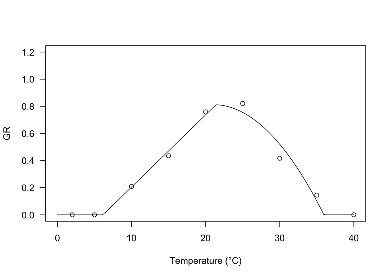
Polynomial model
According to Mesgaran et al (2017), the negative and positive effects of temperature coexist for all temperatures above T_b. Their proposed equation can be parameterised as:
GR = \frac{\max \left[ T, T_b \right] - T_b}{\theta_{T}} \left[ 1 - \frac{\min \left[ T, T_c \right] - T_b}{T_c - T_b} \right] \quad \quad \quad \quad (8)
It is easy to see that the GR value is a second-order polynomial function of T - T_b and, therefore, the curve is symmetric around the optimal temperature value, which can be derived as:
T_o = \frac{T_c - T_b}{2} + T_b
For this equation, the self-starting function is GRT.M().
modM <- drm(GR ~ Tval, fct = GRT.Mb())
plot(modM, log="", xlim = c(0, 40), ylim=c(0,1.2),
     legendPos = c(5, 1.0), xlab = "Temperature (°C)")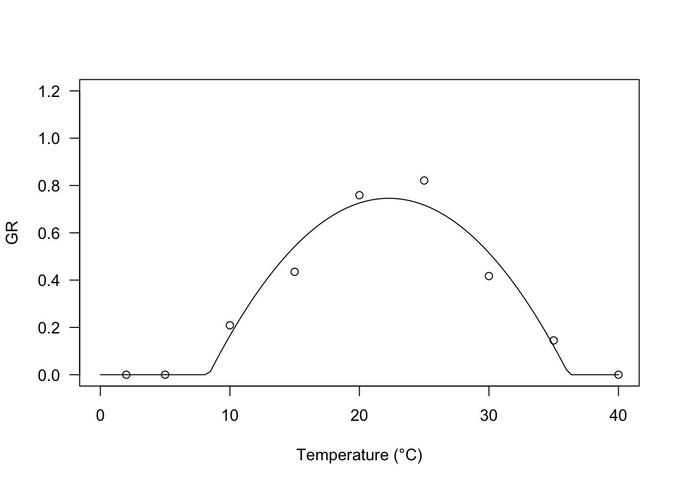
Exponential switch-off model
Equations 6 to 8 use a product, wherein the first term represents the accumulation of thermal time and the second term may be seen as a switch-off term that is 1 either when T < T_o (Equation 6) or T < T_d (Equation 7) or T = T_b (Equation 8) and decreases progressively as temperature increases. In all the above equations, the switch-off term is linear, although we can use other types of switch-off terms, to obtain more flexible models. One possibility is to use an exponential switch-off term, as in the equation below:
GR = \frac{\max \left[T, T_b \right] - T_b}{\theta_T} \left\{ \frac{1 - \exp \left[ k (\min \left[T, T_c \right] - T_c) \right]}{1 - \exp \left[ k (T_b - T_c) \right]} \right\} \quad \quad \quad (9)
where k is the switch-off parameter: the lower the value, the higher the negative effect of temperature at super-optimal levels. The response of GR to temperature is highly asymmetric with a slow increase below T_o and a steep drop afterwards.
I have successfully used this model in Catara et al (2016) and Masin et al (2017). The self-starting function in R is GRT.Exb().
Tval <- c(2, 5, 10, 15, 20, 25, 30, 35, 40)
GR <- c(0, 0, 0.209, 0.435, 0.759, 0.821, 0.917, 0.445, 0)

modExb <- drm(GR ~ Tval, fct = GRT.Exb())
summary(modExb)
##
## Model fitted: Exponential effect of temperature on GR50 (Masin et al., 2017)
##
## Parameter estimates:
##
##                     Estimate Std. Error t-value   p-value
## k:(Intercept)       0.181022   0.060207  3.0067  0.029870 *
## Tb:(Intercept)      5.999610   1.202555  4.9891  0.004143 **
## Tc:(Intercept)     36.937370   0.501322 73.6800 8.724e-09 ***
## ThetaT:(Intercept) 19.159270   2.907228  6.5902  0.001208 **
## ---
## Signif. codes:  0 '***' 0.001 '**' 0.01 '*' 0.05 '.' 0.1 ' ' 1
##
## Residual standard error:
##
##  0.04049371 (5 degrees of freedom)
 r
plot(modExb, log="", xlim = c(0, 40), ylim=c(0,1.2),
     legendPos = c(5, 1.0), xlab = "Temperature (°C)")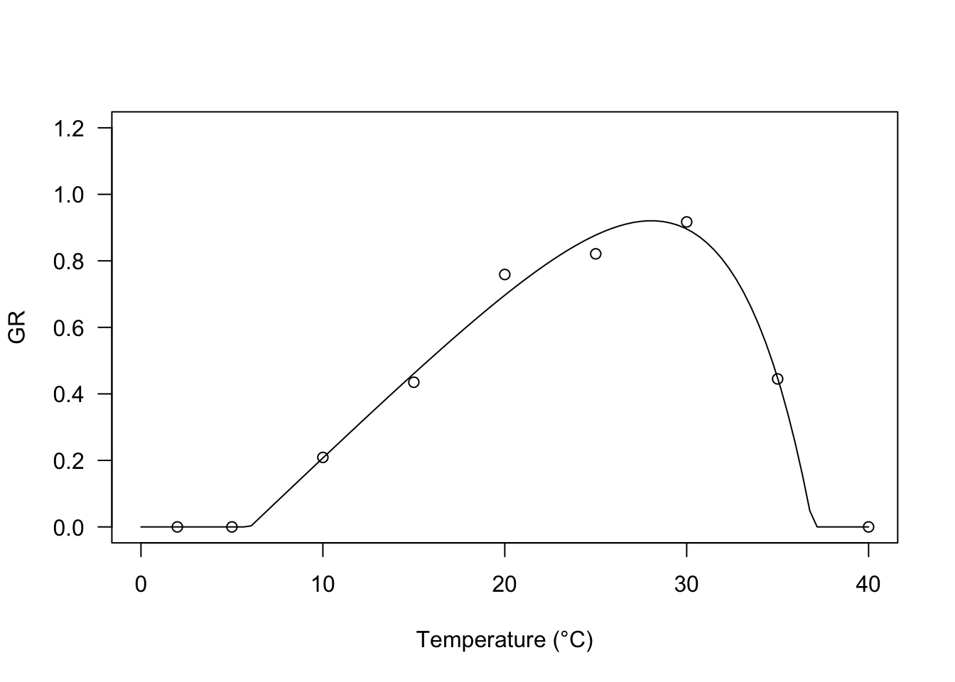
Hyperbolic model
The following model was derived by the simple yield loss function devised by Kropff and van Laar (1993). It is very flexible, as it may depict different types of relationships between temperature and base water potential, according to the value taken by the parameter q.
GR(g, T) = \frac{\max \left[T, T_b\right] - T_b}{\theta_T} \left( 1 - \frac{q \frac{\min \left[T, T_c\right] -T_b}{T_c- T_b} }{1 + (q-1) \frac{T-T_b}{T_c- T_b}} \right) \quad \quad \quad (10)
In R, this model can be fitted by using the self-starter GRT.YL() and we see that, with our dataset, the fit is very much like that of the exponential switch-off function.
modYL <- drm(GR ~ Tval, fct = GRT.YL())
plot(modYL, log="", xlim = c(0, 40), ylim=c(0,1.2),
     legendPos = c(5, 1.0), xlab = "Temperature (°C)")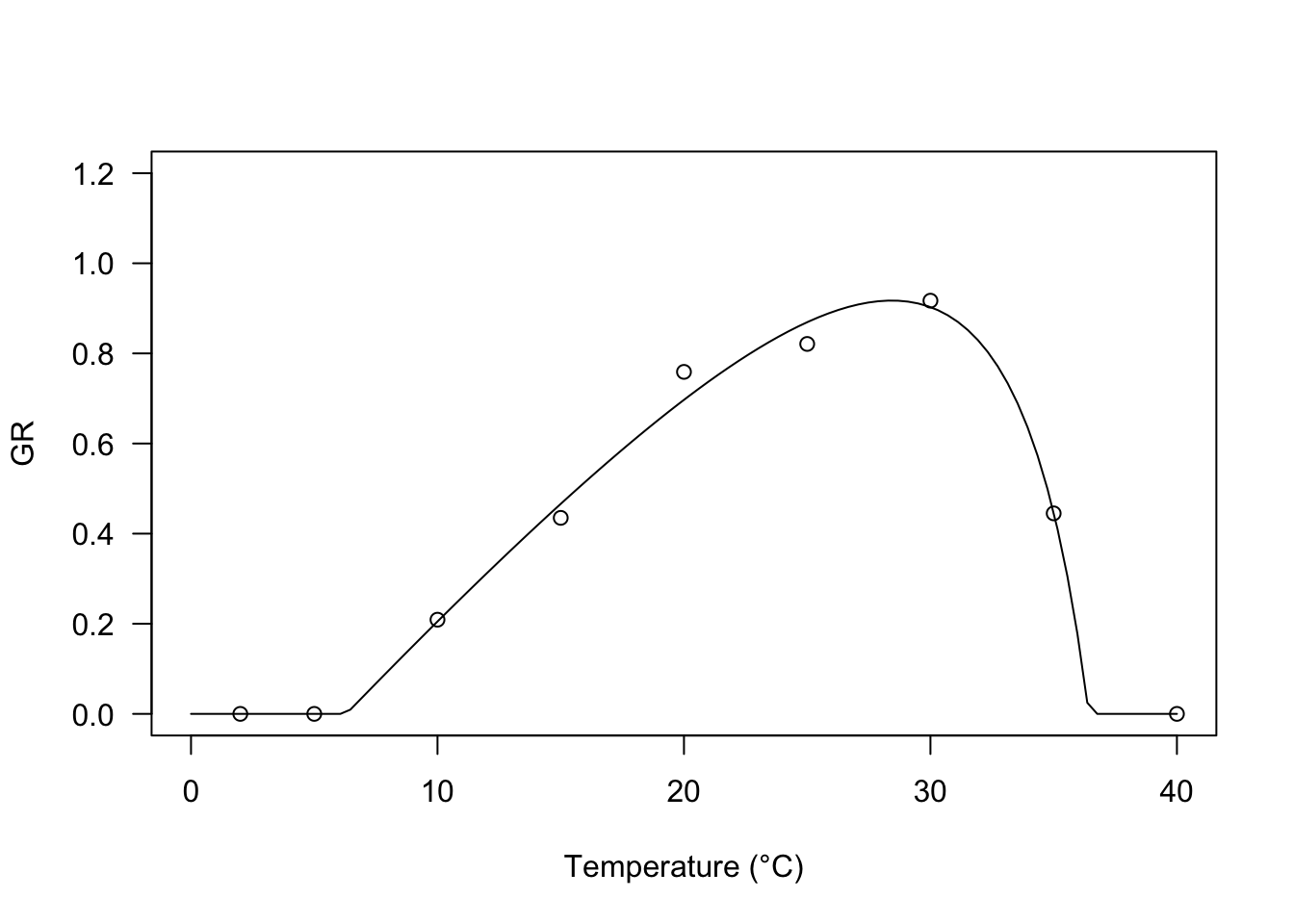
A warning message
When we collect data about the response of germination rates to temperature and use them to parameterise nonlinear regression models by using nonlinear least squares, the basic assumption of homoscedasticity is rarely tenable. We should not forget this! in the above example I used a robust variance-covariance sandwich estimator, although other techniques can be successfully used to deal with this problem.
Thanks for reading and happy coding!
Andrea Onofri
Department of Agricultural, Food and Environmental Sciences
University of Perugia (Italy)
andrea.onofri@unipg.it
References
- Alvarado, V., Bradford, K.J., 2002. A hydrothermal time model explains the cardinal temperatures for seed germination. Plant, Cell and Environment 25, 1061–1069.
- Baty, F., Ritz, C., Charles, S., Brutsche, M., Flandrois, J. P., Delignette-Muller, M.-L., 2014. A toolbox for nonlinear regression in R: the package nlstools. Journal of Statistical Software, 65, 5, 1-21.
- Bradford, K.J., 2002. Applications of hydrothermal time to quantifying and modelling seed germination and dormancy. Weed Science 50, 248–260.
- Catara, S., Cristaudo, A., Gualtieri, A., Galesi, R., Impelluso, C., Onofri, A., 2016. Threshold temperatures for seed germination in nine species of Verbascum (Scrophulariaceae). Seed Science Research 26, 30–46.
- Garcia-Huidobro, J., Monteith, J.L., Squire, R., 1982. Time, temperature and germination of pearl millet (Pennisetum typhoides S & H.). 1. Constant temperatures. Journal of Experimental Botany 33, 288–296.
- Kropff, M.J., van Laar, H.H. 1993. Modelling crop-weed interactions. CAB International, Books.
- Masin, R., Onofri, A., Gasparini, V., Zanin, G., 2017. Can alternating temperatures be used to estimate base temperature for seed germination? Weed Research 57, 390–398.
- Onofri A., 2019. DrcSeedGerm: Statistical approaches for data analyses in seed germination assays. R package version 0.98. https://www.statforbiology.com
- Onofri, A., Benincasa, P., Mesgaran, M.B., Ritz, C., 2018. Hydrothermal-time-to-event models for seed germination. European Journal of Agronomy 101, 129–139.
- Ritz, C., Jensen, S. M., Gerhard, D., Streibig, J. C., 2019. Dose-Response Analysis Using R. CRC Press
- Rowse, H.R., Finch-Savage, W.E., 2003. Hydrothermal threshold models can describe the germination response of carrot (Daucus carota) and onion (Allium cepa) seed populations across both sub- and supra-optimal temperatures. New Phytologist 158, 101–108.
- Zeileis, A., 2006. Object-oriented computation of sandwich estimators. Journal of Statistical Software, 16, 9, 1-16.